gggenomes - a multi-track ggplot2 extension for comparative genomics • gggenomes

gggenomes is an extension to ggplot2 tailored to the visualization of genomics data. It provides the same flexible approach for building up plots layer by layer, but supports the simultaneous use of multiple datasets within one plot, thereby intuitively mirroring the relational nature of most ’omics data products.

A ggplot2 is build around a single, tidy dataset with arbitrary variables and observations. x/y-plot coordinates for things to draw are computed on-the-fly using aesthetic mappings that link variables to coordinates. This setup is highly flexible and makes ggplot extremely powerful.

A gggenomes plot is build around multiple data tracks that each contain a single dataset. These datasets are linked via pre-computed global layout that determines x/y-plot coordinates prior to the actual plot construction. The reason for this more rigid setup is that genomics data are relational and there is just no good way to represent all the necessary information in a single tidy table.

gggenomes knows three types of tracks:

seqs: sequences such as contigs or chromosomes
feats: annotations of locations on sequences, such genes, SNPs, …
links: annotations that connect two locations between two different sequences

There are also genes tracks, those, however are just glorified feature tracks, that sometimes get special treatment for easier usage. Internally, genes are features.

library(gggenomes)

# a minimal seq track
s0 <- tibble::tibble(
  seq_id = c("a", "b"),
  length = c(600, 550)
)

# a minimal gene track
g0 <- tibble::tibble(
  seq_id = c("a", "a", "b"),
  start = c(50, 350, 80),
  end = c(250, 500, 450)
)

# a simple link track
l0 <- tibble::tibble(
  seq_id = c("a", "a"),
  start = c(50, 400),
  end = c(250, 480),
  seq_id2 = c("b", "b"),
  start2 = c(80, 350),
  end2 = c(300, 430)
)

p <- gggenomes(genes=g0, seqs=s0, links=l0)
p + 
  geom_seq() +         # draw contig/chromosome lines
  geom_seq_label() +   # label each sequence 
  geom_gene() +        # draw genes as arrow
  geom_link()          # draw some connections between syntenic regions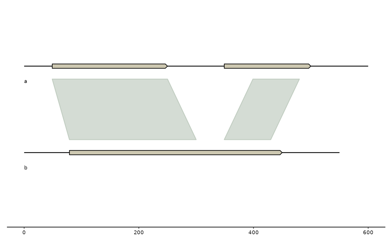

Geoms and tracks

In a regular ggplot2, geoms read from one central dataframe. For gggenomes, there are several tracks to read data from. To specify which tracks to use in which geoms, gggenomes provides accessory functions that work inside geom calls when provided to the data argument (or outside if prefixed with pull_). The names of these functions mirror the track types they work on and should be quite intuitive:

geom_seq() : data=seqs() for the seq track
geom_feat() : data=feats() for the first feat track not named “genes”
geom_link() : data=links() for the first link track
geom_gene() : data=genes() for the first feat track with some extras for geneish features (see Inside gggenomes tracks for details)

gggenomes supports an arbitrary number of feature and link tracks within the same plot. Extra tracks can be added by either providing a list of tracks to gggenomes(), or by using the dedicated add_feats() / add_links() functions. The extra tracks can then be used via the aforementioned accessory function inside geom calls using names or positional arguments. Like most gggenomes functions the track accessory functions use tidyverse-style non-standard evaluation, which means you can refer to tracks either by unquoted names or by numeric position.

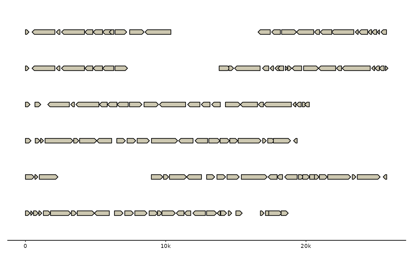
# Let's use some of the bundled example data here
data(package="gggenomes")

p <- gggenomes(
  genes=emale_genes,  # a gene track, added as first feat track
  seqs=emale_seqs,    # a seq track
  feats=list(emale_tirs, emale_ngaros),  # multiple feat tracks
  links=emale_ava     # a link track
)

# inspect the tracks of the plot
p %>% track_info

## # A tibble: 5 × 4
## # Groups:   type [3]
##   id           type      i     n
##   <chr>        <chr> <int> <int>
## 1 seqs         seqs      1     6
## 2 genes        feats     1   143
## 3 emale_tirs   feats     2    12
## 4 emale_ngaros feats     3     3
## 5 links        links     1    38

# plot all tracks
p +
#  geom_link() +  # the first link track
  geom_gene() +  # the first feat track filtered for geneish feats: CDS, mRNA, ..
  geom_feat() +  # the first feat track not named "genes", here emale_tirs
  # use an extra feat track by name
  geom_feat(data=feats(emale_ngaros), color="plum3")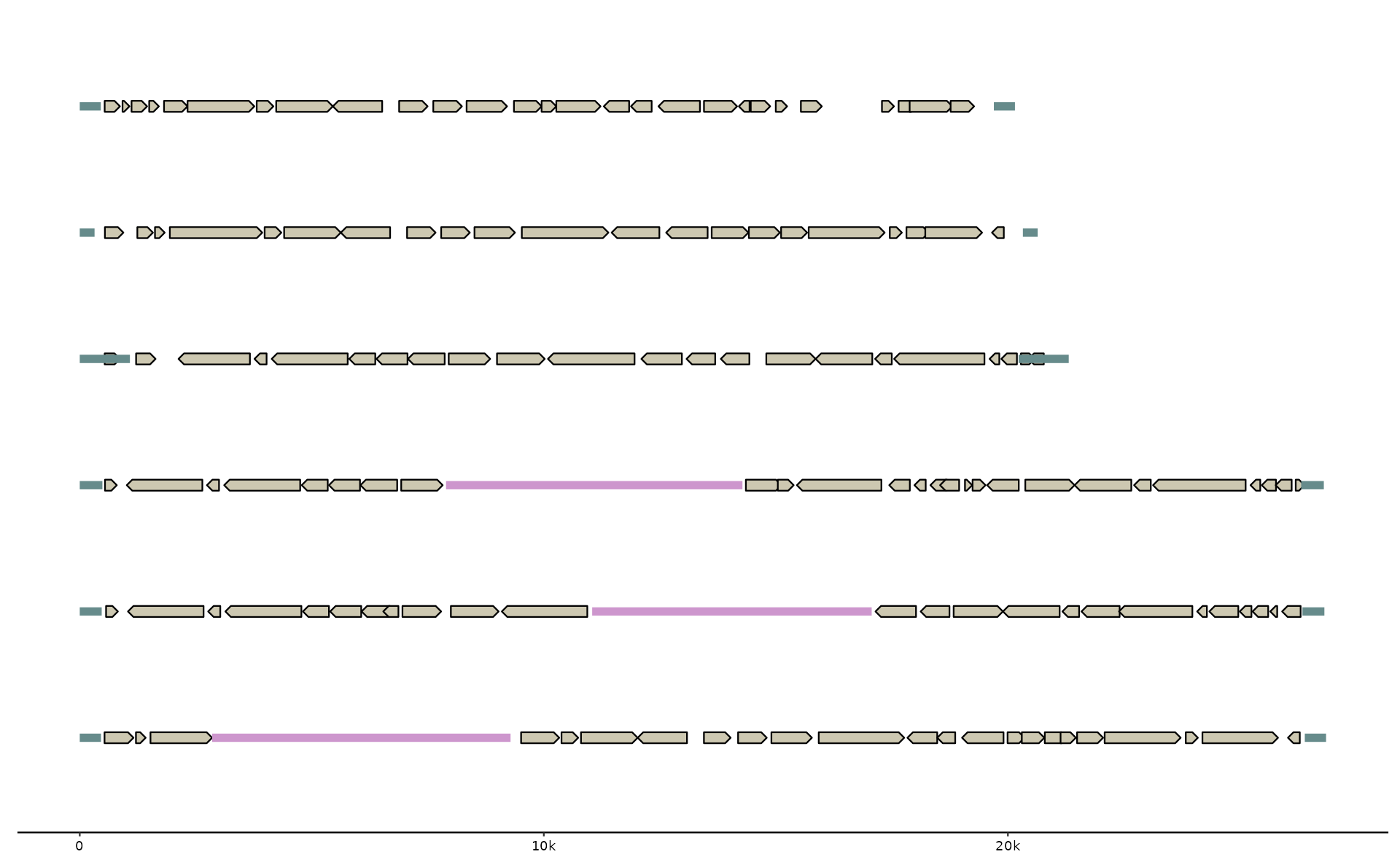

One layout to rule them all

gggenomes multi-track setup has both pros and cons. For example, communicating information between tracks during plot construction is not supported by ggplot2, because - well - it’s been designed to work with a single table. gggenomes works around that by pre-computing a layout, and adding coordinates (y,x,xend) to each dataframe prior to the actual plot construction. This has some implications for the usage of gggenomes:

Dataframes for tracks have required variables, e.g. seq_id,start,end for features. These predefined variables are used during import to compute x/y coordinates (see Inside gggenomes tracks for more details).
gggenomes geoms can often be used without explicit aes() mappings - a rather convenient upside of the multi-track setup. This works because we always know the names of the plot variables ahead of time: they originate from the pre-computed layout, and we can use that information to set sensible default aesthetic mappings for most cases.

# inspect seqs track with layout vars - note y,x,xend
p %>% pull_seqs

## # A tibble: 6 × 12
## # Groups:   bin_id [6]
##       y     x  xend strand seq_id   bin_id length bin_offset start   end file_id
##   <int> <dbl> <dbl> <chr>  <chr>    <chr>   <int>      <dbl> <dbl> <int> <chr>  
## 1     6     0 20152 +      RCC970_… RCC97…  20152          0     1 20152 emales 
## 2     5     0 20642 +      E4-10_0… E4-10…  20642          0     1 20642 emales 
## 3     4     0 21311 +      Cflag_0… Cflag…  21311          0     1 21311 emales 
## 4     3     0 26808 +      BVI_069  BVI_0…  26808          0     1 26808 emales 
## 5     2     0 26820 +      BVI_008A BVI_0…  26820          0     1 26820 emales 
## 6     1     0 26856 +      E4-10_1… E4-10…  26856          0     1 26856 emales 
## # ℹ 1 more variable: seq_desc <chr>

# inspect genes track with layout vars - note y,x,xend, but also other
# columns such as strand, feat_id or type, that are added automatically
p %>% pull_genes

## # A tibble: 143 × 22
##        y     x  xend bin_id   seq_id   start   end file_id strand type  feat_id 
##    <int> <dbl> <dbl> <chr>    <chr>    <int> <int> <chr>   <chr>  <chr> <chr>   
##  1     2   567   822 BVI_008A BVI_008A   568   822 emales  +      CDS   BVI_008…
##  2     2  2668  1039 BVI_008A BVI_008A  1040  2668 emales  -      CDS   BVI_008…
##  3     2  3028  2767 BVI_008A BVI_008A  2768  3028 emales  -      CDS   BVI_008…
##  4     2  4776  3138 BVI_008A BVI_008A  3139  4776 emales  -      CDS   BVI_008…
##  5     2  5370  4809 BVI_008A BVI_008A  4810  5370 emales  -      CDS   BVI_008…
##  6     2  6065  5396 BVI_008A BVI_008A  5397  6065 emales  -      CDS   BVI_008…
##  7     2  6683  6074 BVI_008A BVI_008A  6075  6683 emales  -      CDS   BVI_008…
##  8     2  6867  6540 BVI_008A BVI_008A  6541  6867 emales  -      CDS   BVI_008…
##  9     2  6954  7788 BVI_008A BVI_008A  6955  7788 emales  +      CDS   BVI_008…
## 10     2  7997  9026 BVI_008A BVI_008A  7998  9026 emales  +      CDS   BVI_008…
## # ℹ 133 more rows
## # ℹ 11 more variables: introns <list>, parent_ids <list>, source <chr>,
## #   score <chr>, phase <int>, width <chr>, gc_content <chr>, name <chr>,
## #   Note <chr>, geom_id <chr>, .marginal <lgl>

Plotting from scratch

The minimum requirement to create a gggenomes plot is a single track. It can be of any of the three types: seqs, feats or links.

If there is no a sequence track, a sequence track is inferred from the data simply by assuming that each sequence that a feature or link maps onto must exist, and that it must be long enough to accommodate all its associated features and links (note the corresponding log message below).

Note also, that unless sequence information is explicitly provided, gggenomes will zoom in on only the regions that are covered with features. That may appear odd at first, but it is a) consistent in the sense that for inferred sequence we only know the start (x=1) anyway, and have to guess the end from the last feature, and b) it is very convenient if we deal with real data: It usually makes no sense to plot all 5000 genes of a bacterial genome. In most cases we will want to focus on specific regions.

# some genes
g0 <- tibble::tibble(
  seq_id = c("a", "a", "b"),
  start = c(50, 350, 80),
  end = c(250, 500, 450)
)

p <- gggenomes(g0)

## No seqs provided, inferring seqs from feats

p +
  geom_seq() +         # draw contig/chromosome lines
  geom_seq_label() +   # label each sequence 
  geom_gene()          # draw genes as arrow

## Only saw `type=NA` in genes and will treat everything as `type="CDS"`.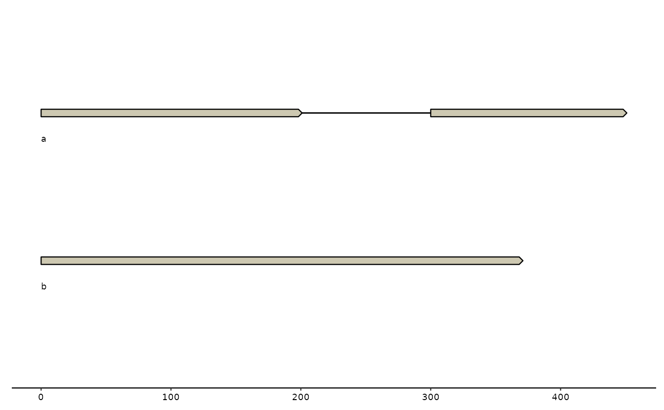

Plotting from files

Plotting from scratch is fun, but likely not the typical use-case. Usually you will have files with data that you want to import. gggenomes provides a bunch of read_* functions that help you do that for several common bioinformatics file formats. Moreover, gggenomes come with a set of higher-level convenience read functions that perfectly integrate with its track system.

What I mean by that is that instead of reading a certain file format explicitly, such as read_gff3("foo.gff"), you can invoke the generic read_feats("foo.gff") function to read features from various file formats. File formats are automatically recognized, so this, for example, also works read_feats("foo.bed"). And you can read different information from the same file: read_seqs("foo.gff") will retrieve sequence information from the gff3 file instead of gene/feature coordinates.

That said, the only real requirement for any data you want to plot is that it is in a somewhat tidy table, and that it has some of the required variables (see below). Even if you have data that is not directly supported by gggenomes read functions, it should be very easy to convert your data into a table that works with gggenomes.

# note: ex() is just a helper to get stable paths to gggenomes example data
s0 <- read_seqs(ex("emales/emales.fna"))
g0 <- read_feats(ex("emales/emales.gff"))

gggenomes(g0, s0) +
  geom_seq() + geom_gene()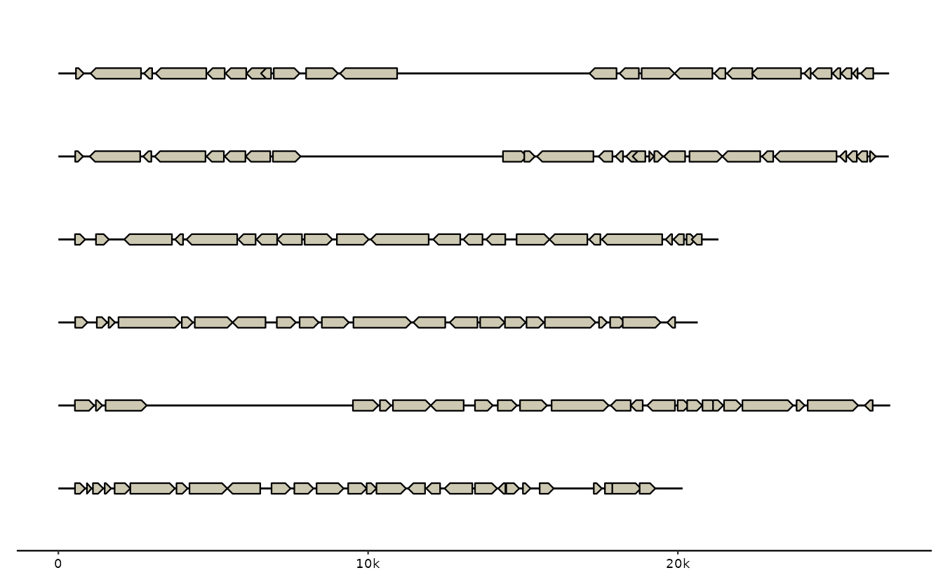

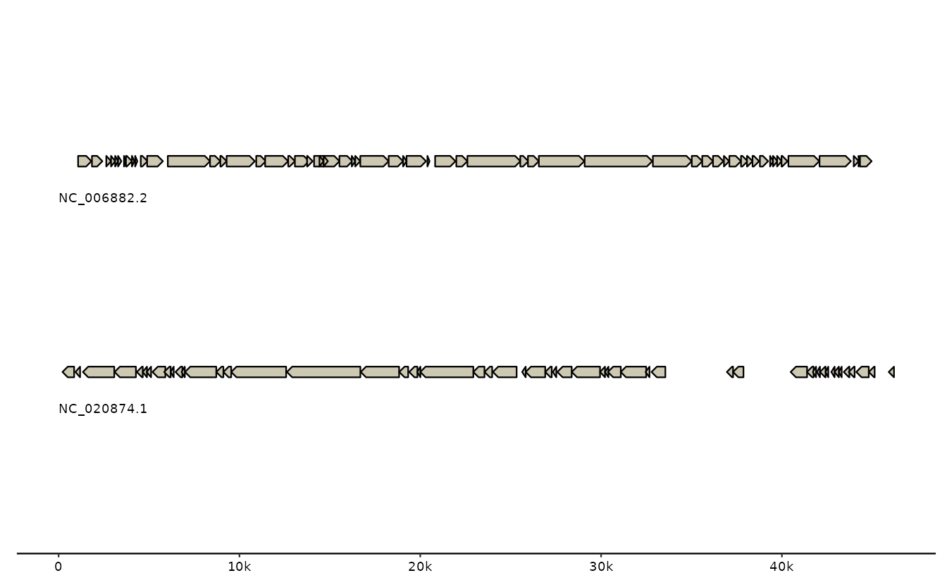
# for lazy people
gggenomes(ex("emales/emales.gff")) + geom_gene()

# and really fancy: multiple remote files, all at once
gbk_phages <- c(
  PSSP7 = "ftp://ftp.ncbi.nlm.nih.gov/genomes/all/GCF/000/858/745/GCF_000858745.1_ViralProj15134/GCF_000858745.1_ViralProj15134_genomic.gff.gz",
  PSSP3 = "ftp://ftp.ncbi.nlm.nih.gov/genomes/all/GCF/000/904/555/GCF_000904555.1_ViralProj195517/GCF_000904555.1_ViralProj195517_genomic.gff.gz")
gggenomes(gbk_phages) + geom_gene() +
  geom_seq_label()

Inside gggenomes tracks

As mentioned before, tracks have required columns and optional columns, which can have additional meaning in the context of the plot.

seqs: sequences such as contigs or chromosomes

required: seq_id,length
recognized: bin_id,start,end,strand

feats: such as genes, SNPs, repeats, …

required: seq_id,start,end
recognized: strand,bin_id,feat_id,introns

links: connections between two locations from different sequences

required: seq_id,seq_id2
recognized: start,end,bin_id,start2,end2,bin_id2,strand

Sequence track - there can be only one

seq_id,length are the required variables and should be quite self-explanatory. It’s highly recommended (and might become compulsory in the future) for seq_ids to be unique within the entire data set.

The optional column for seqs are:

bin_id to denote bins representing genomes or assemblies with multiple chromosomes or contigs. Sequences from the same bin are drawn next to each other in the default layout, as opposed to sequence from different bins which will occupy different rows. If omitted, the default is to set bin_id=seq_id, which means, every sequence gets its own row.

# seq track: one entry per sequence
s0 <- tibble::tibble(
  bin_id = c("A", "A", "B"),
  seq_id = c("a1","a2","b1"),
  length = c(2e5, 3e5, 5e5)
)

p <-  gggenomes(seqs=s0) 
p +
  geom_seq() +         # draw contig/chromosome lines
  geom_seq_label()    # label each sequence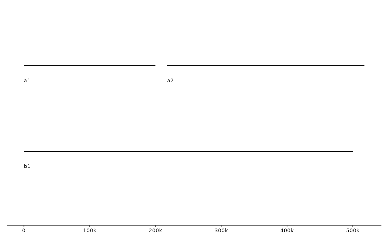

  #geom_bin_label()  # label each bin

start,end,strand in the context of a sequence denote a region or locus on that sequence. If provided, only the part of the sequence within the locus boundaries will be shown in the plot. This also will remove any features from the plot that do not fall within the locus. It’s likely rare to one wants to specify these information directly, but they are important as they power manipulation functions such as focus().

# zoom in on a longer sequence - note the scale on the x-axis
s0 <- tibble::tibble(
  seq_id = "a1",
  length = 10000,
  start = 1000,
  end = 3000
)
gggenomes(seqs=s0) + geom_seq() + geom_seq_label()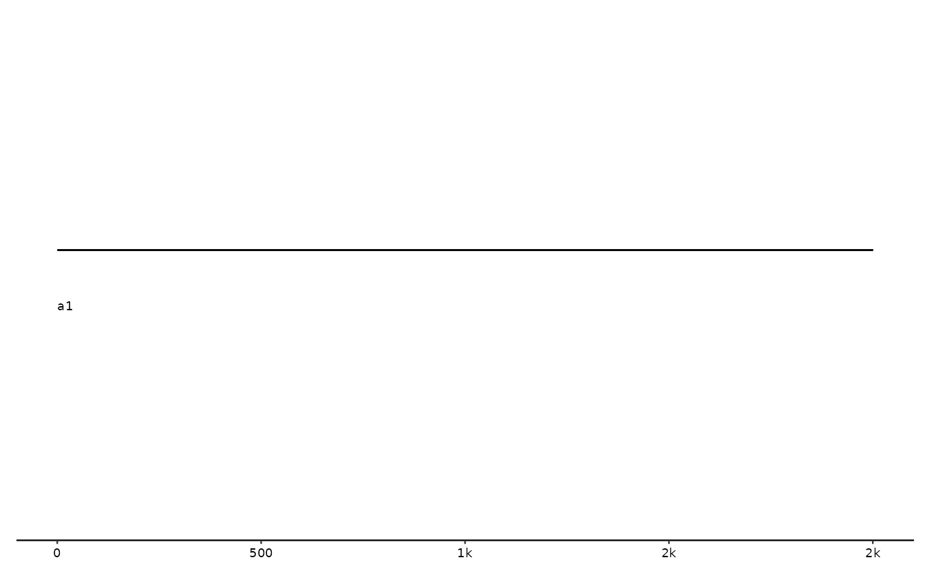

Feature tracks - what maps onto sequences

Again, the required variables seq_id,start,end should be self-explainatory. Note though, that features with seq_ids not present in the seq track will be silently ignored.

Also note that gggenomes uses 1-based, inclusive ranges to denote feature start/end coordinates. It’s the same system as used by GFF, GenBank, BLAST or SAM, for example. In contrast, BED and BAM, for example, use 0-based, exclusive ranges. Something to keep in mind when importing data from those formats.

The optional columns for features are:

strand to denote the orientation of a feature relative to the sequences it maps to. The default way of specifying the strand is with a character vector with "+/-/." coding for forward, reverse and undetermined. Logical (TRUE/FALSE/NA) or numeric vectors (1/-1/0) are supported as well.

bin_id works as for seqs. The assignment of bin_ids to features is usually only useful, if no sequences are provided. Otherwise, bin information is inherited from the sequences.

feat_id is a unique ID for each feature. These IDs are useful if we want to add data to a plot that pertains to features and not sequences. For example, we can add the results of a protein blast search to the genes the proteins derived from if by matching blast results and feature annotations using the feat_id. If not provided, they will be automatically generated.

Special variables for complex gene models:

introns is a special column that can contain a list of numeric vectors that denote intron start and end coordinates within a given feature. The support of introns is something I just very recently added. It’s still experimental and some of the handling might change in future versions.

# some genes
g0 <- tibble::tibble(
  seq_id = c("a"),
  start = c(1, 800),
  end = c(500, 1200),
  # NOTE: introns need to be a list-column!
  introns = list(c(50,200), c(50,200,250,300))
)

gggenomes(g0) +
  geom_seq() +         # draw contig/chromosome lines
  geom_seq_label() +   # label each sequence 
  geom_gene()          # draw genes as arrow

## No seqs provided, inferring seqs from feats
## Only saw `type=NA` in genes and will treat everything as `type="CDS"`.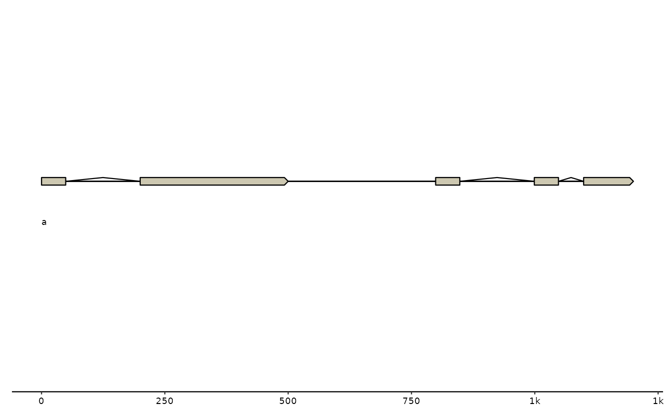

Link tracks - show me the synteny

The link track connects loci/regions on two adjacent sequences/genomes with one another. seq_id, seq_id2 are the required variables for the link track. Once again, links with seq_ids not present in the sequence (seq) track will be silently ignored.
To correctly link specific loci/regions between sequences with one another, it is also highly recommend to use the following optional variables: (Without the variables, start, start2,endandend2`, links will be made between two entire sequences/contigs and not between two specific loci/regions.)

start, start2 indicates the starting position of the loci/region that will be linked between respectively the first sequence (seq_id) and the second sequence (seq_id2). Note that links can and will only be created between adjacent sequences.

end, end2 similar to start and start2, but now indicates the end of the loci/region that will be linked. Once again respectively for seq_id and seq_id2.

bin_id, bin_id2 works as for seqs. The assignment of bin_ids to features is usually only useful, if no sequences are provided. Otherwise, bin information is inherited from the sequences.

strand, works as for feats. strand denotes the orientation of the link relative to each of the two sequences. If abscent, the orientation is derived from the start and end positions.

# some links
l0 <- tibble::tibble(
  seq_id = c("a", "a", "a"),
  start = c(200, 801, 1600),
  end = c(550, 1300, 1800),
  seq_id2 = c("b", "b", "b"),
  start2 = c(1100, 1, 1800),
  end2 = c(1450, 500, 1600)
)

# corresponding sequences
s1 <- tibble::tibble(
  seq_id = c("a", "b"), 
  length = c(2000, 2000),
  start = c(1, 1),
  end = c(2000, 2000)
)


gggenomes(seqs=s1, links=l0)  +
  geom_seq() +                  # draws contigs/chromosome lines  
  geom_seq_label()             # labels each sequence

 # geom_link(offset = 0.05)      # draws links between contigs

gggenomes - a multi-track ggplot2 extension for comparative genomics

Thomas Hackl

2/23/2021