geom_variant allows the user to draw points at locations where a mutation has occurred. Data on SNPs, Insertions, Deletions and more (often stored in a variant call format (VCF)) can easily be visualized this way.
Usage
geom_variant(
  mapping = NULL,
  data = feats(),
  stat = "identity",
  position = "identity",
  geom = "variant",
  na.rm = FALSE,
  show.legend = NA,
  inherit.aes = TRUE,
  offset = 0,
  ...
)
Arguments
- mapping
Set of aesthetic mappings created by
aes(). If specified andinherit.aes = TRUE(the default), it is combined with the default mapping at the top level of the plot. You must supplymappingif there is no plot mapping.- data
Data from the first feats track is used for this function by default. When several feats tracks are present within the gggenomes track system, make sure that the wanted data is used by calling
data = feats(*df*)within thegeom_variantfunction.- stat
Describes what statistical transformation is used for this layer. By default it uses
"identity", indicating no statistical transformation.- position
Describes how the position of different plotted features are adjusted. By default it uses
"identity", but different position adjustments, such asposition_variant(), ggplot2'"jitter"or"pile"can be used as well.- geom
Describes what geom is called upon by the function for plotting. By default the function uses
"variant", a modified geom_point object. For larger sequences with abundant mutations/variations, it is recommended to use"ticks"(a modified geom_point object with different default shape and alpha, which plots the points as small "ticks"), but in theory any other ggplot2 geom can be called here as well.- na.rm
If
FALSE, the default, missing values are removed with a warning. IfTRUE, missing values are silently removed.- show.legend
logical. Should this layer be included in the legends?
NA, the default, includes if any aesthetics are mapped.FALSEnever includes, andTRUEalways includes. It can also be a named logical vector to finely select the aesthetics to display. To include legend keys for all levels, even when no data exists, useTRUE. IfNA, all levels are shown in legend, but unobserved levels are omitted.- inherit.aes
If
FALSE, overrides the default aesthetics, rather than combining with them. This is most useful for helper functions that define both data and aesthetics and shouldn't inherit behaviour from the default plot specification, e.g.annotation_borders().- offset
Numeric value describing how far the points will be drawn from the base/sequence. By default it is set on
offset = 0.- ...
Other arguments passed on to
layer()'sparamsargument. These arguments broadly fall into one of 4 categories below. Notably, further arguments to thepositionargument, or aesthetics that are required can not be passed through.... Unknown arguments that are not part of the 4 categories below are ignored.Static aesthetics that are not mapped to a scale, but are at a fixed value and apply to the layer as a whole. For example,
colour = "red"orlinewidth = 3. The geom's documentation has an Aesthetics section that lists the available options. The 'required' aesthetics cannot be passed on to theparams. Please note that while passing unmapped aesthetics as vectors is technically possible, the order and required length is not guaranteed to be parallel to the input data.When constructing a layer using a
stat_*()function, the...argument can be used to pass on parameters to thegeompart of the layer. An example of this isstat_density(geom = "area", outline.type = "both"). The geom's documentation lists which parameters it can accept.Inversely, when constructing a layer using a
geom_*()function, the...argument can be used to pass on parameters to thestatpart of the layer. An example of this isgeom_area(stat = "density", adjust = 0.5). The stat's documentation lists which parameters it can accept.The
key_glyphargument oflayer()may also be passed on through.... This can be one of the functions described as key glyphs, to change the display of the layer in the legend.
Details
geom_variant uses ggplot2::geom_point under the hood. As a result, different aesthetics such as alpha, size, color, etc.
can be called upon to modify the data visualization.
#' the function gggenomes::read_feats is able to read VCF files and converts them into a format that is applicable within the gggenomes' track system.
Keep in mind: The function uses data from the feats' track.
Examples
# Creation of example data.
# (Note: These are mere examples and do not fully resemble data from VCF-files)
## Small example data set
f1 <- tibble::tibble(
seq_id = c(rep(c("A", "B"), 4)), start = c(1, 10, 15, 15, 30, 40, 40, 50),
end = c(2, 11, 20, 16, 31, 41, 50, 51), length = end - start,
type = c("SNP", "SNP", "Insertion", "Deletion", "Deletion", "SNP", "Insertion", "SNP"),
ALT = c("A", "T", "CAT", ".", ".", "G", "GG", "G"),
REF = c("C", "G", "C", "A", "A", "C", "G", "T")
)
s1 <- tibble::tibble(seq_id = c("A", "B"), start = c(0, 0), end = c(55, 55), length = end - start)
## larger example data set
f2 <- tibble::tibble(
seq_id = c(rep("A", 667)),
start = c(
seq(from = 1, to = 500, by = 2),
seq(from = 500, to = 2500, by = 50),
seq(from = 2500, to = 4000, by = 4)
),
end = start + 1, length = end - start,
type = c(
rep("SNP", 100),
rep("Deletion", 20),
rep("SNP", 180),
rep("Deletion", 67),
rep("SNP", 100),
rep("Insertion", 50),
rep("SNP", 150)
),
ALT = c(
sample(x = c("A", "C", "G", "T"), size = 100, replace = TRUE),
rep(".", 20), sample(x = c("A", "C", "G", "T"), size = 180, replace = TRUE),
rep(".", 67), sample(x = c("A", "C", "G", "T"), size = 100, replace = TRUE),
sample(x = c(
"AA", "AC", "AG", "AT", "CA", "CC", "CG", "CT", "GA", "GC",
"GG", "GT", "TA", "TC", "TG", "TT"
), size = 50, replace = TRUE),
sample(x = c("A", "C", "G", "T"), size = 150, replace = TRUE)
)
)
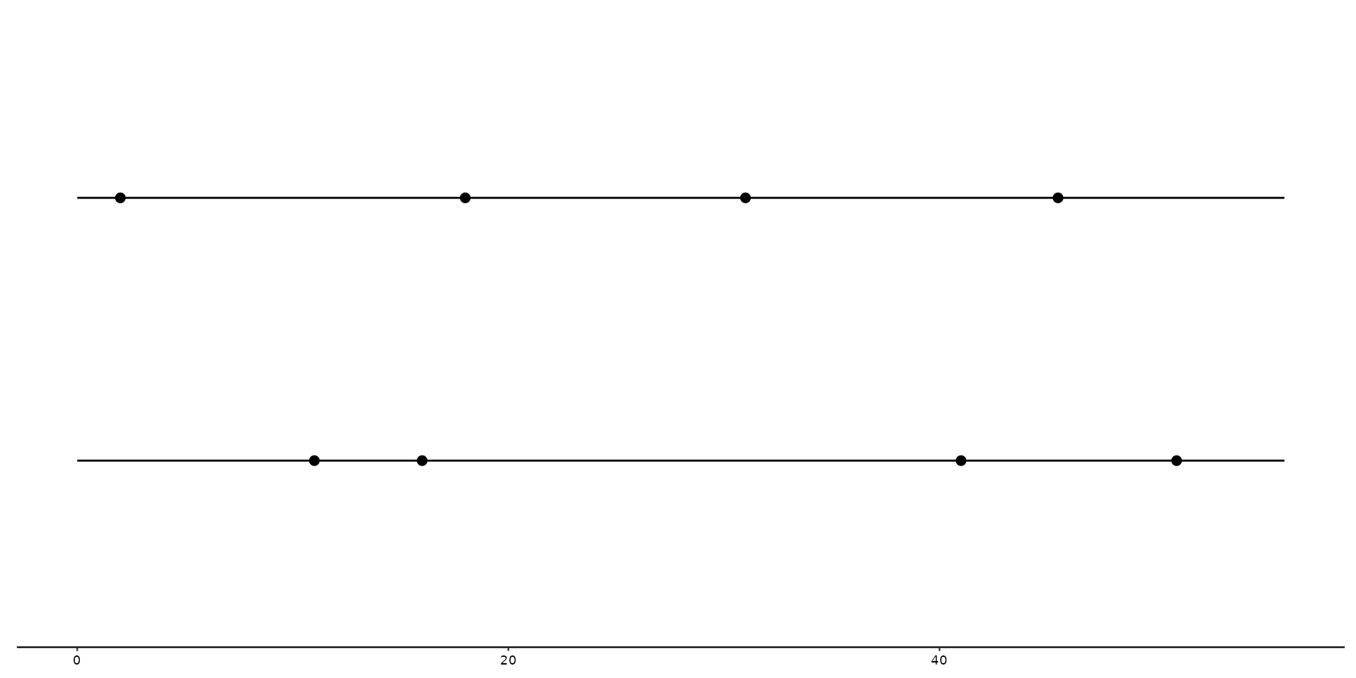
# Basic example plot with geom_variant
gggenomes(seqs = s1, feats = f1) +
geom_seq() +
geom_variant()
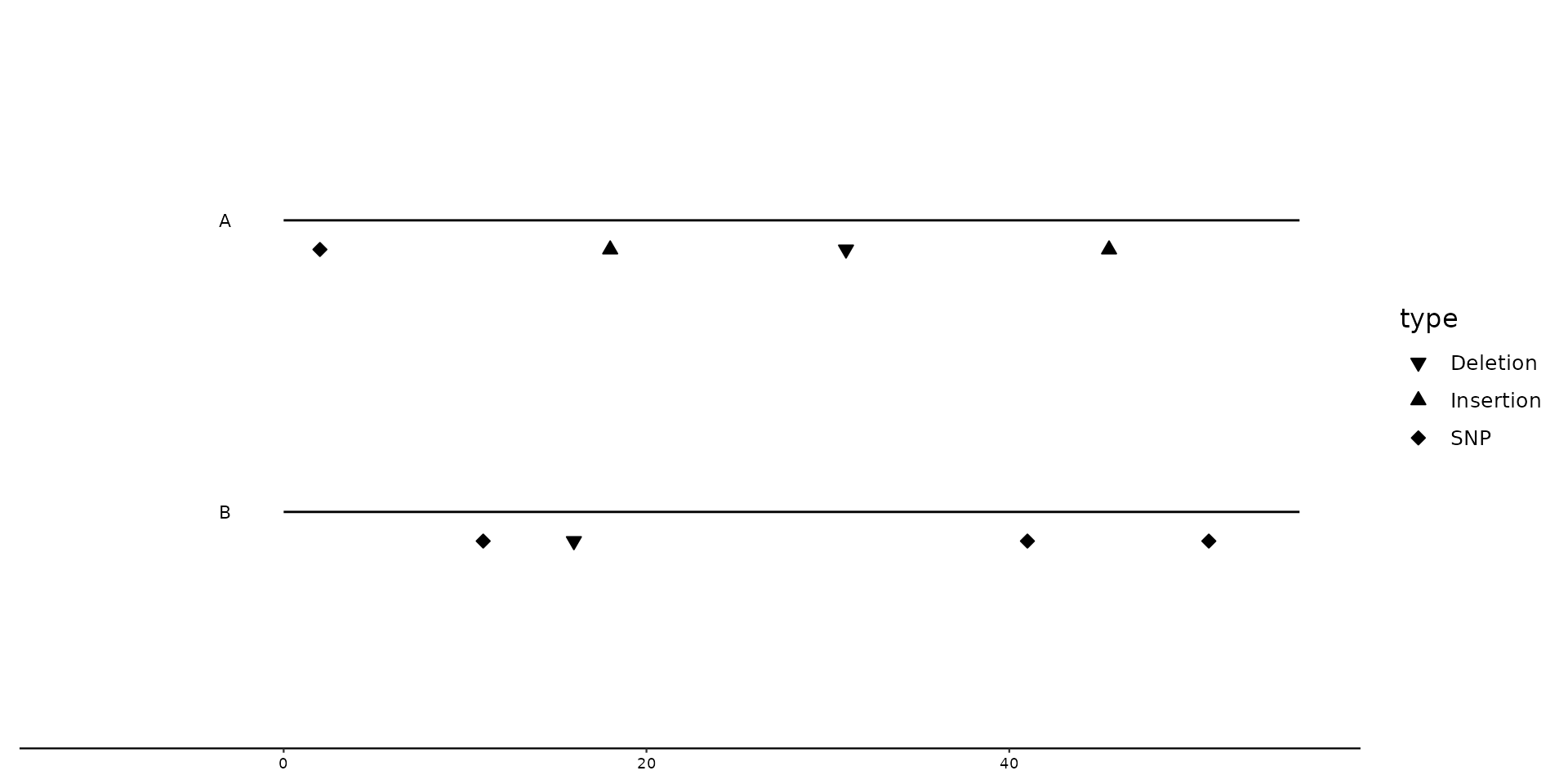
 # Improving plot elements, by changing shape and adding bin_label
gggenomes(seqs = s1, feats = f1) +
geom_seq() +
geom_variant(aes(shape = type), offset = -0.1) +
scale_shape_variant() +
geom_bin_label()
# Improving plot elements, by changing shape and adding bin_label
gggenomes(seqs = s1, feats = f1) +
geom_seq() +
geom_variant(aes(shape = type), offset = -0.1) +
scale_shape_variant() +
geom_bin_label()
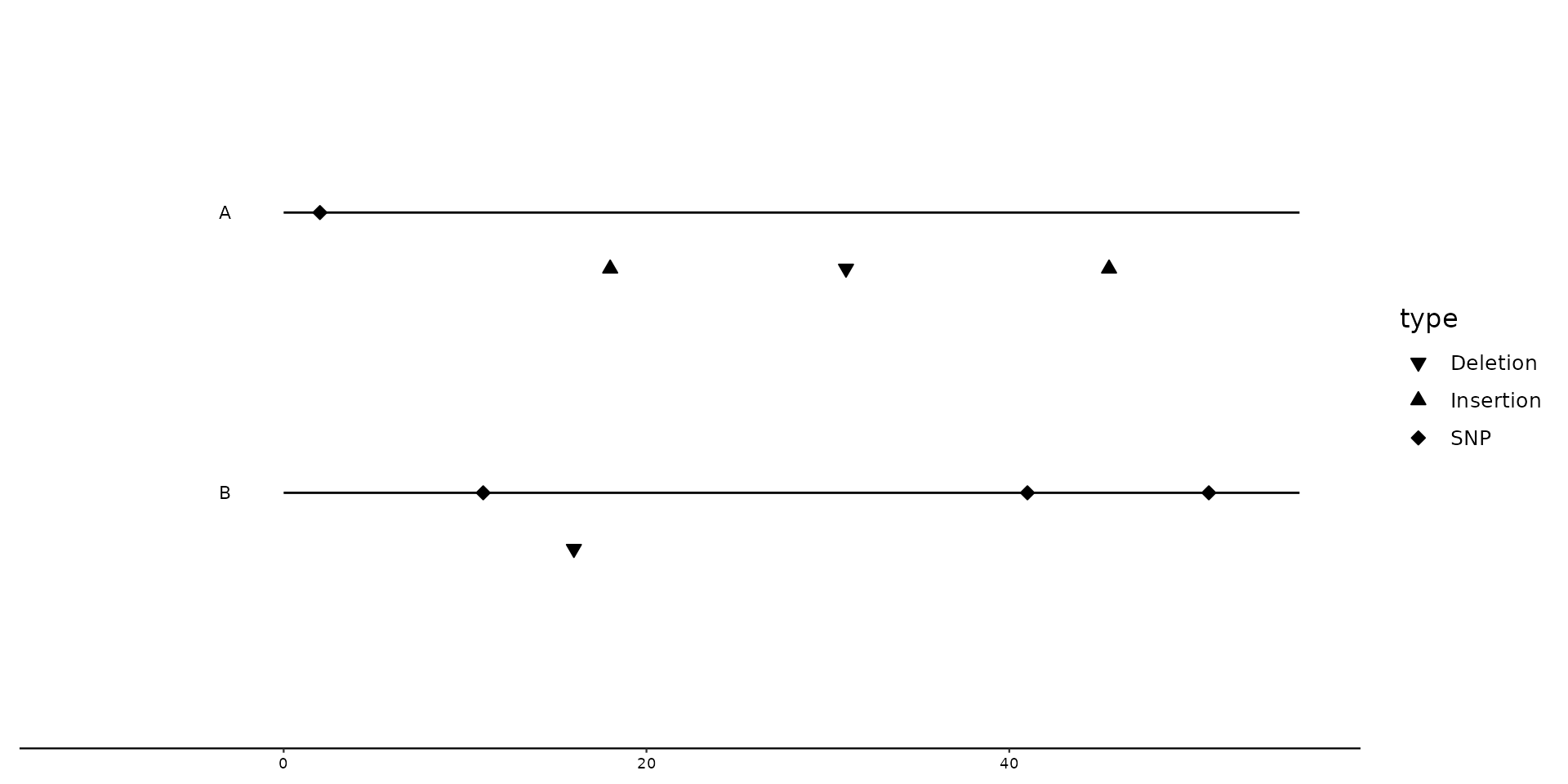
 # Positional adjustment based on type of mutation: position_variant
gggenomes(seqs = s1, feats = f1) +
geom_seq() +
geom_variant(
aes(shape = type),
position = position_variant(offset = c(Insertion = -0.2, Deletion = -0.2, SNP = 0))
) +
scale_shape_variant() +
geom_bin_label()
# Positional adjustment based on type of mutation: position_variant
gggenomes(seqs = s1, feats = f1) +
geom_seq() +
geom_variant(
aes(shape = type),
position = position_variant(offset = c(Insertion = -0.2, Deletion = -0.2, SNP = 0))
) +
scale_shape_variant() +
geom_bin_label()
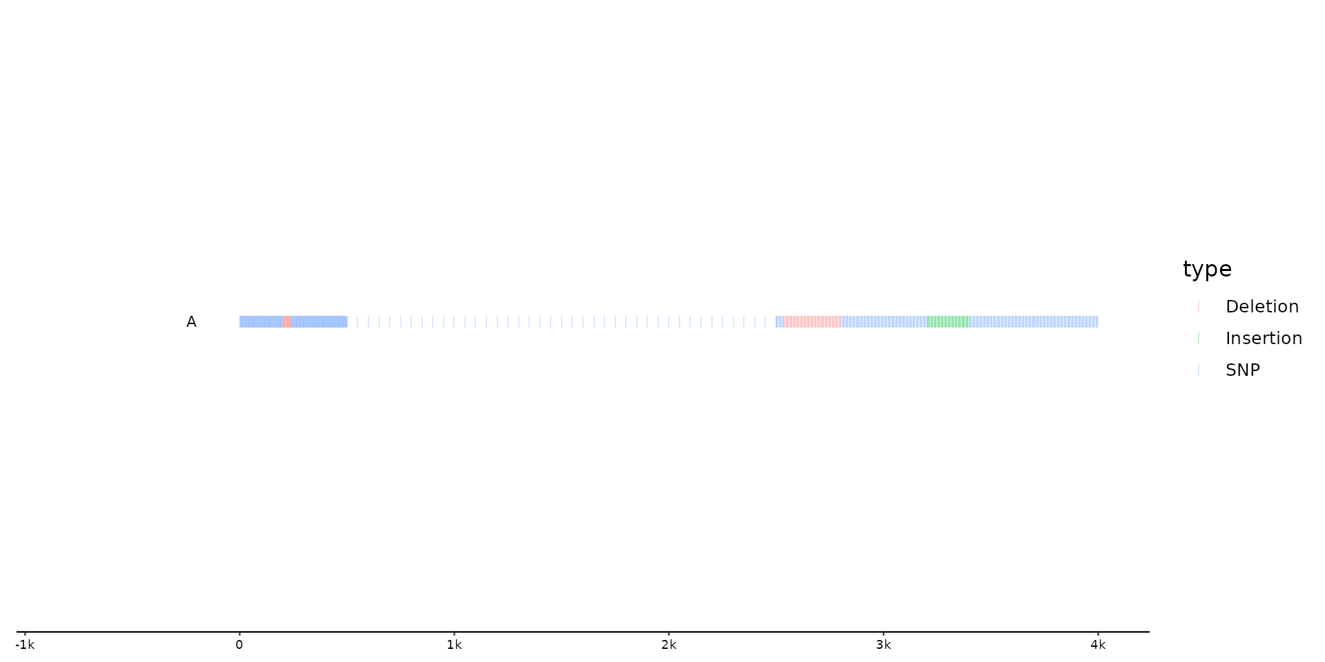
 # Plotting larger example data set with Changing default geom to
# `geom = "ticks"` using positional adjustment based on type (`position_variant`)
gggenomes(feats = f2) +
geom_variant(aes(color = type), geom = "ticks", alpha = 0.4, position = position_variant()) +
geom_bin_label()
#> No seqs provided, inferring seqs from feats
#> Warning: Some mutation types are not mentioned within the offset argument. These types will have an offset of 0 by default
# Plotting larger example data set with Changing default geom to
# `geom = "ticks"` using positional adjustment based on type (`position_variant`)
gggenomes(feats = f2) +
geom_variant(aes(color = type), geom = "ticks", alpha = 0.4, position = position_variant()) +
geom_bin_label()
#> No seqs provided, inferring seqs from feats
#> Warning: Some mutation types are not mentioned within the offset argument. These types will have an offset of 0 by default
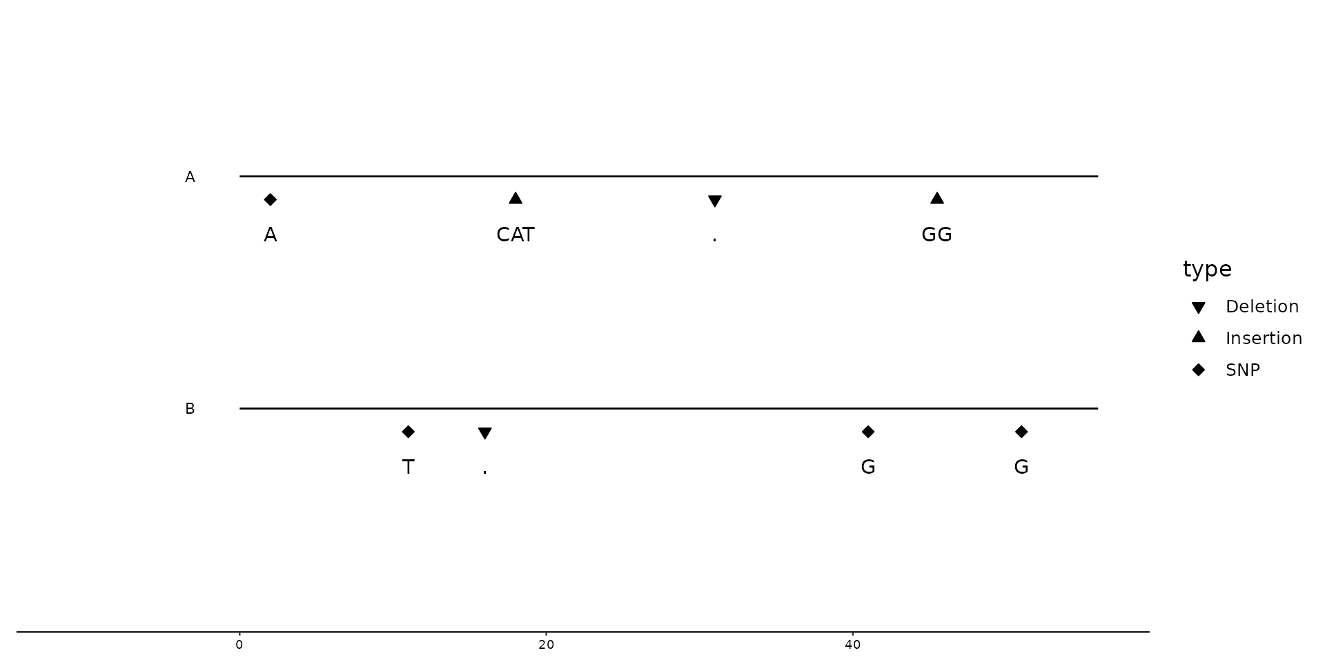
 # Changing geom to `"text"`, to plot ALT nucleotides
gggenomes(seqs = s1, feats = f1) +
geom_seq() +
geom_variant(aes(shape = type), offset = -0.1) +
scale_shape_variant() +
geom_variant(aes(label = ALT), geom = "text", offset = -0.25) +
geom_bin_label()
#> Warning: Ignoring unknown aesthetics: type
# Changing geom to `"text"`, to plot ALT nucleotides
gggenomes(seqs = s1, feats = f1) +
geom_seq() +
geom_variant(aes(shape = type), offset = -0.1) +
scale_shape_variant() +
geom_variant(aes(label = ALT), geom = "text", offset = -0.25) +
geom_bin_label()
#> Warning: Ignoring unknown aesthetics: type